
Maximum Day Demand and Capital Investment Decisions
Capital investment for water networks routinely reaches tens of millions of dollars - and often hundreds.
A new pipeline over a long distance is necessary.
The pump station and storage tank need upgrading as well.
And expensive rock excavation is required too.
You get the point.
The cost hinges on two things. First, demand i.e. how much water will the new development actually use?
The second parameter is timing.
In Net Present Value terms, money spent years from now costs far less in today's dollars.
So where the demand data justifies deferring the works, the saving is real.
Deciding how big to build, and when, is exactly where SCADA data mining earns its value.
Where the demand numbers come from
The demand numbers behind capital decisions at utilities have historically come from the source data - the flow measured at the treatment plant or dam.
In decades past this made sense as the source was the only usable data, and subsystem/zone level monitoring was only beginning in the early 2000s.
But across a large network with many distinct supply zones, the source data captures only a single system-wide average - and misses the spatial variability of demand across vast areas.
Residential demand varies from zone to zone because of differences in housing footprints, socioeconomics, appliance efficiency and water restrictions - and day to day temperature and rainfall too. Commercial and industrial demand also varies from zone to zone.
Source data smooths all of that into one number - but it's the variation from the average that determines whether you can safely defer capital expenditure, or reduce utility risk.
SensorClean's data mining shows the demand in each zone which can improve capital decisions, supported by new demand evidence.
Maximum Day Demand in the observed record
SensorClean defines the Maximum Day Demand as the highest consumption day - following data cleaning - that is in the observed SCADA record.
Figure 1 shows about 10 years of data for four example subsystems.
You will notice that the Maximum Day Demand (shown in red) does not occur on the same day.
Similarly, the Maximum Week Demand does not occur at the same time in these subsystems.
This means that only relying on source data for modeling, does not reveal the reality of demand variability and therefore misses opportunities to reduce risk and save on capital expenditure.
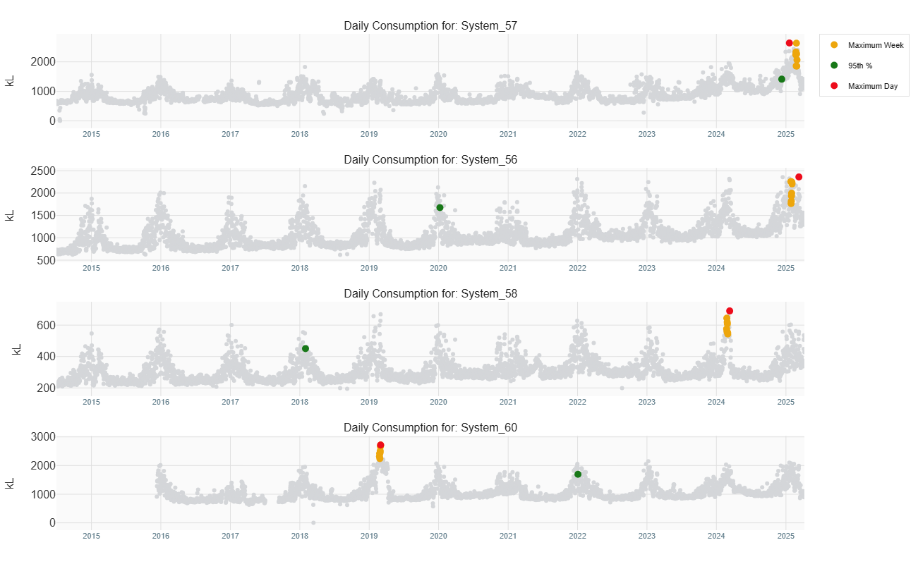
Figure 1 Timing of Maximum Day Demand for four example subsystems/zones in a water distribution system
Maximum Day Demand and weather uplift
In demand analysis for capital decisions, it’s important to separate the weather signal – temperature and rainfall - from the underlying water usage.
Without doing this, a run of hot summers can look like demand growth - and you size capital infrastructure for demand that isn't there.
Strip the weather out, and what's left is the underlying community demand, with insights about how it might be changing.
If the weather normalized Maximum Day Demand has an increasing trend, then this can be accounted for in demand projections for future infrastructure.
Figure 2 shows the weather normalized Maximum and Average Day Demand for example Subsystem 21 – which is a rural subsystem with a 99% residential contribution. This provides a simplification of the analysis by assuming that commercial and industrial components are insignificant.
Two things stand out in Figure 2:
the weather normalized Average Day trend is steady and well-fitted (R² = 0.80) - demand is rising consistently.
The weather normalized Maximum Day trend is noisier (R² = 0.34), because maximum days are event-driven — they depend on how many hot, dry days a given summer happened to deliver.
Weather normalization is what lets you see the trend beneath that noise.
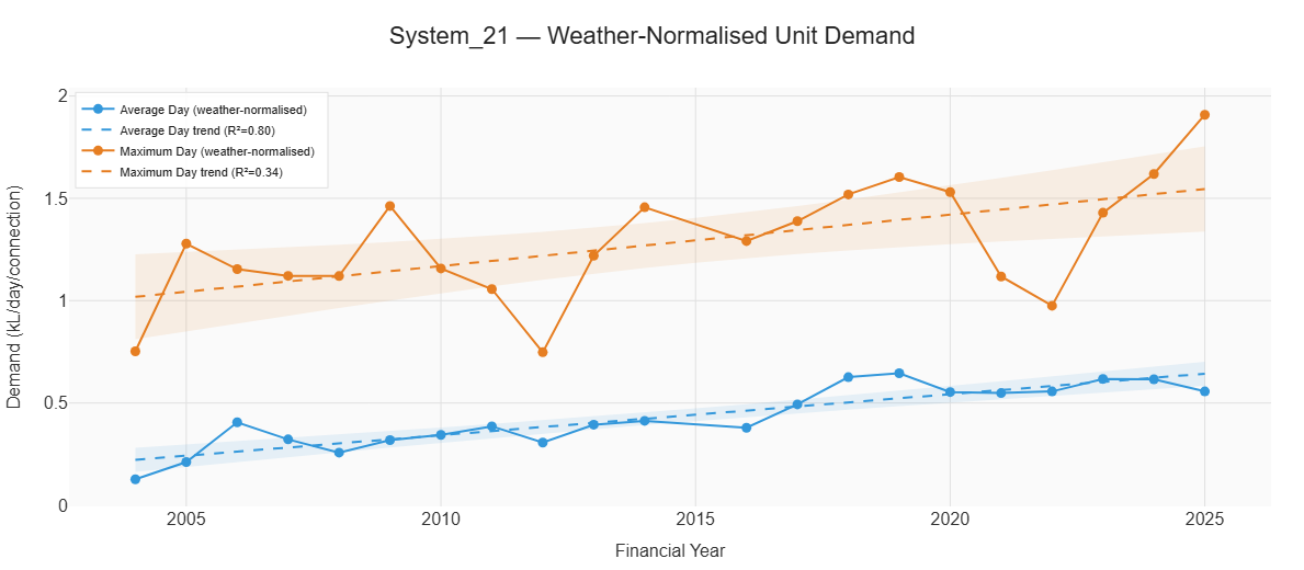
Figure 2 Weather-normalized Maximum and Average Day Demand per connection for example subsystem 21
Where utilities supply historical connection data - for example from staged development shapefiles - SensorClean incorporates per-year connection counts directly into the demand timeline. That separates change in community demand from growth in connection numbers.
SensorClean also analyses night flow trends to ensure we’re not designing for existing leakage growth.
Climate change loading
If the weather-normalized Maximum Day Demand is increasing, that can be carried into demand projections for future infrastructure.
In addition, future warming scenarios can be added - modeling what a warmer climate would add to Maximum Day Demand, with the uncertainty quantified to support robust decision-making.
Figure 3 shows the three components for an example demand projection, which is:
Weather normalized Maximum Day Demand in the observed SCADA records
Underlying demand changes using the trend in Figure 2
Climate loading under an example 2°C warming scenario
For subsystem 21, the observed Maximum Day Demand of 1.908 kL/day/connection projects to 2.356 by 2040.
Most of that increase comes from underlying growth in community demand; the climate loading under 2°C warming is a comparatively small addition.
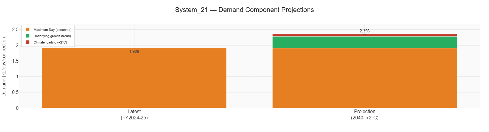
Figure 3 Example subsystem 21 with observed Maximum Day Demand (weather normalized) with projected demand growth and 2°C climate loading to 2040.
The projected demand in Figure 3 along with a normalized Maximum Day Demand diurnal profile can be used in modeling future subsystems.
If profiles are required at the level of houses and apartments, regression can be used for profile development (see blog).
There is also the possibility, that behaviour in response to weather will change as higher temperatures are normalized e.g. gardens will be planted with less thirsty vegetation.
Peak Day Demand for design purposes
Peak Day Demand is the term used by utilities for design purposes and is most commonly linked to source data.
In Australia, it is calculated by taking the Average Day Demand — in kiloliters per day per connection - and then scaling it up using a peaking factor to give the Peak Day Demand. Commercial and industrial demands are treated separately and are often not considered to be ‘too peaky’.
For example, a residential house with a backyard (and garden) may have a peaking factor of 2.25 which means the design demand is set at 2.25 times the projected average day demand.
The value in seeing Maximum Day Demand metrics for many subsystems is that you can compare them with your design Peak Day Demand to get some notion of whether a subsystem has either:
Observed demand that sits below the design Peak Day - the design was conservative, there's headroom, and capital works may be deferrable
Observed demand that exceeds the design Peak Day - the design underestimated real demand, and there's risk to address
Observed and design align - the "do nothing" answer, still valuable because it confirms the assumption and prevents a poor decision
Conclusion
Data mining at the subsystem level reveals new evidence about demand variability across a water network - evidence that helps planners reduce risk and avoid over-spending on capital works.
When comparing legacy source-data metrics against subsystem mining, design flows turn out to be higher, lower, or about right - and knowing which, before committing tens of millions is what data mining delivers.
If you'd like to see what your own subsystem data reveals, get in touch.