
What Minimum Night Flows Tell You About Leakage
Water loss from aging infrastructure, commonly referred to as non-revenue water, is estimated to cost global taxpayers more than USD 39 billion per year (Liemberger and Wyatt 2019).
In Australia, the median water loss across utilities of all sizes is 72 liters per connection per day (Bureau of Meteorology 2024).
For a utility with 100,000 connections, that equates to approximately 2.6 billion liters of lost water each year.
While large pipe failures attract media attention and lose considerable volumes of water, it is the low-level background leakage that quietly accumulates into significant losses over time.
SCADA monitoring systems - implemented in Australia since the late 1990s - already collect vast amounts of operational data from water supply networks.
When analyzed beyond traditional spreadsheet workflows, utilities can use this data to prioritize maintenance interventions where they will deliver the greatest return on investment.
For example, Figure 1 illustrates a District Metered Area (DMA) ranking derived from SCADA data mining, providing maintenance teams with clear, data-driven priorities for reducing water loss.
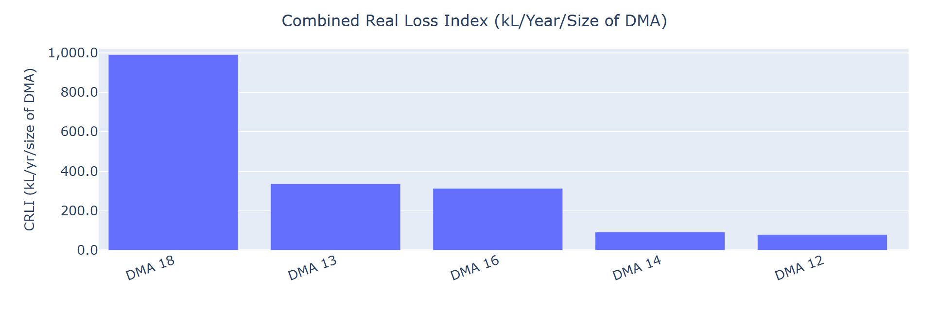
Figure 1 Normalized leakage estimates providing maintenance teams with the greatest opportunity to reduce leakage. The Combined Real Loss Index (kiloliter/year/size of DMA) is used, as it captures both high-density urban and rural DMAs.
Without structured SCADA data prioritization, utilities risk directing maintenance resources to the wrong parts of the network.
Interrogating minimum night flows
A commonly used indicator of leakage is change in the Minimum Night Flow (MNF).
Utilities have relied on MNF analysis for decades because water demand is typically lowest during the early hours of the morning, when most customers are asleep.
These low-flow periods provide the clearest signal of background leakage within a distribution network.
At a seasonal scale, night flows are generally higher during summer than winter. In Australia, this is often due to off-peak irrigation and sprinkler use.
As a result, seasonal context should always be considered when interpreting MNF trends.
Annual lowest night flows
To understand how night flows are changing within a DMA, a practical and defensible reference point is the lowest credible night flow observed in each year — referred to as the Annual Lowest Night Flow (ALNF).
However, not every low reading is credible as SCADA data is inherently variable.
For this reason, annual lowest night flows cannot reliably be selected using algorithms alone (more on this below).
SensorClean’s workflow supports a structured, human-in-the-loop approach by presenting engineers with candidate days for each year. Users can:
See the relationship between daily MNF, temperature, and rainfall
View the off-peak window with both raw and smoothed traces
Check surrounding diurnal profiles for operational context
Compare multiple candidate days
Apply engineering judgment before confirming the ALNF.
In the example video (2024), candidate low-flow days are displayed so they can be interrogated visually.
You may notice that off-peak data often contains noise - which is why a 15-minute rolling smoother is applied to aid interpretation.
Automation will continue to improve, particularly through AI agents trained on this methodology. However, at present, robust and defensible results require structured night flow analysis supported by engineering judgment.
Only after this quality assurance process can a day be confirmed as that year’s ALNF.
Video 1 Annual Lowest Night Flow (ALNF) candidate selection for 2024.
Video Description: The video presents four candidate days for the Annual Lowest Night Flow (ALNF) in 2024. The view initially shows surrounding diurnal profiles to provide operational context, before zooming into the off-peak period for detailed analysis. Both raw and smoothed traces are displayed to support interpretation. On-screen text explains that if Candidate 1 is deemed erroneous based on engineering judgment, an alternative candidate (e.g., Candidate 2) can be selected as the ALNF.
Selecting a baseline to quantify leakage
Figure 2 shows a night flow timeline for a DMA – displaying daily MNFs and daily maximum temperature - with annotated Annual Lowest Night Flows (ALNFs) that have been checked with quality assurance.
The next step is to select one of these values as the baseline, so leakage growth can be quantified.
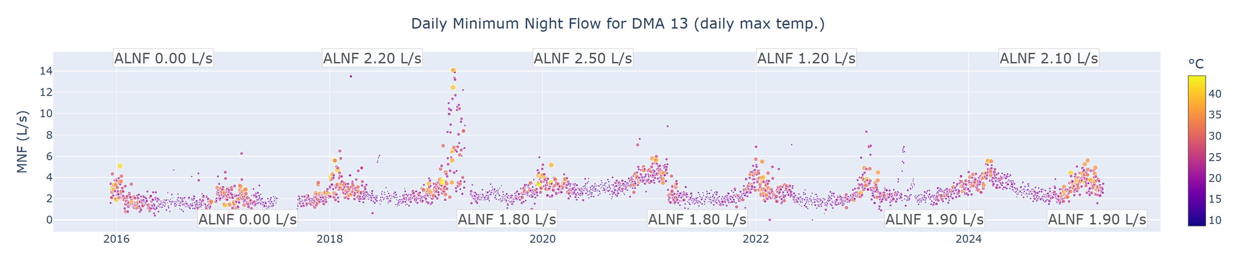
Figure 2 Timeline of daily minimum night flows with the selected annual lowest night flows.
In the night flow timeline, there appears to be a structural change in night flows in 2020 where the ALNF was the highest on record at 2.5 L/s.
It is possible that maintenance fixed a leak (in early 2021) resulting in a return to 1.8 L/s in 2021. Baseline selection should therefore occur from 2021 onward.
Only complete data years should be used for baseline selection, which excludes 2025 from Figure 2. For analyzing night flows for incomplete or ‘current’ years we suggest weekly checking with a seasonal night flow model (see blog).
For baseline selection of DMA 13 in Figure 2, we are therefore left with:
2021 ALNF of 1.8 L/s
2022 ALNF of 1.2 L/s
2023 ALNF of 1.9 L/s; and
2024 ALNF of 2.1 L/s.
As the lowest credible ALNF within this period is 1.2 L/s in 2022, this value becomes the DMA’s baseline (Figure 3).
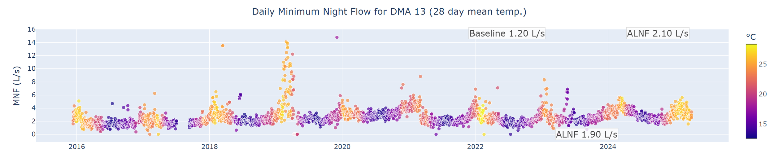
Figure 3 Night Flow Timeline with Baseline Selection
As new data becomes available, additional ALNFs are confirmed. If a new credible ALNF lower than the current baseline is observed — for example following a leak repair — the baseline should be updated accordingly.
With the selected ALNFs and baseline confirmed, a clear timeline of system performance can be established, as shown in Figure 3.
Maintenance interventions can be overlaid onto this timeline to assess their effectiveness and quantify performance improvements.
Year-over-year leakage growth can be estimated, providing an evidence base for maintenance prioritization and capital planning.
Known development changes can also be incorporated. For example, the connection of a laundromat may permanently increase night flows and should be flagged for decision-makers when interpreting shifts in night flow behavior.
Calendar years vs financial years
Defining “year” requires seasonal consideration.
In Australia, financial years run from July 1 to June 30. However, because the lowest night flows typically occur in mid-winter (June–August), using calendar years provides clearer seasonal grouping when visualizing and selecting annual candidates.
Grouping by calendar year prevents winter low-flow periods from being split across reporting windows and makes year-to-year comparison more consistent and intuitive.
Why simple automation fails
It is tempting to automate ALNF selection using rules such as:
Analyzing the 1:00 am–5:00 am window
Applying a rolling smoother (e.g. 15-minute median); and
Selecting the 1st or 2nd percentile over a five-year period.
In practice, this approach leads to errors.
The reason is that SCADA night flow data is highly variable across systems.
A percentile threshold that works for one DMA may fail for another.
Percentile-based selection can capture erroneous or non-representative data, while also missing credible low-flow conditions that require visual and operational review.
There is no single statistical rule that consistently identifies credible lowest flow conditions across diverse systems.
Smart meters and leakage
The scale of global water loss has helped drive widespread agreement that residential smart meters are an important part of the future.
Established benefits include:
Identification of leaks between the meter and the property
Improved water awareness through consumption-tracking applications; and
Removal of manual meter readings.
At the network scale, if a DMA has full smart meter coverage and all meters record simultaneously, leakage can be estimated with high accuracy.
However, published evidence of large-scale network leakage reduction attributed to smart meter rollout remains limited.
While smart meters offer clear customer leak and demand reduction benefits, utilities already possess extensive SCADA data – that when cleaned and organized – can deliver actionable network leakage insights today.
Smart meters are future-enabling for network leakage analytics.
Cleaned SCADA data is immediately actionable.
Conclusion
By interrogating night flows with engineering rigor and structured SCADA analysis, utilities can move from reactive leak response to proactive leakage management.
If you want to quantify leakage growth and identify the highest-return interventions in your network, let’s review your SCADA data together.
References
Bureau of Meteorology (2024), National performance report 2022–23: urban water utilities, part A, Bureau of Meteorology, Melbourne
Liemberger, R. and A. Wyatt (2019). "Quantifying the global non-revenue water problem." Water Supply 19(3): 831–837.